Decision Trees

Overview

Decision trees are a popular machine learning algorithm that can perform both classification and regression tasks. Decision trees create a model that predicts the value of a target variable by learning simple decision rules inferred from the data features. The decision tree splits the data based on the most significant variable at each node. Then the algorithm generates a tree structure where each leaf node represents a class or a regression value. The decision tree algorithm decides which feature to split the data at each node and measures the split quality based on a criterion such as Gini impurity, Entropy, or Information Gain.

Gini, Entropy, and Information Gain

The Gini impurity measures the probability of misclassification if a random element from the subtree Child nodes with a lower Gini impurity than the parent node results from a good split. The Gini impurity ranges from 0 (no impurity) to 1 (most impurity). If i is a class label, $C$ is the total number of classes, and $p_i$ is the relative frequency of class $i$ in the node:

$\text{Gini} = 1 - \sum_{i=1}^C p_i^2$

Entropy is another criterion used to measure the impurity of a set of labels. Like with the Gini impurity, child nodes with lower entropy than the parent node result from a good split. It measures the disorder or uncertainty within a label set.

$\text{Entropy} = \sum_{i=1}^C -p_i\log_2(p_i)$

Information gain is a metric that measures the reduction in entropy or Gini impurity achieved by a split. We can calculate the Gini impurity by subtracting the weighted impurity of the child nodes from the impurity of the parent node. The node split with the highest information gain is then selected.

In the example below the Gini impurity for the ‘Low’ node with 4 total observations can be calculated by:

$\text{Gini}(\text{Low}) = 1 - \left((\frac{3}{4})^2 + (\frac{1}{4})^2\right) = 0.37$

Once the individual Gini impurities are calculated for each node, the information gain is:

$\text{Information Gain} = \text{Gini}(\text{Income}) - \sum_{j=1}^N p_j \cdot\text{Gini}(j) \\ = \text{Gini}(\text{Income}) - \left((\frac{2+2}{14})0.5 + (\frac{4+2}{14})0.44 + (\frac{3+1}{14})0.37\right) = 0.44$

Where $j$ is a child node, $N$ is the number of child nodes, and $p_j$ is the frequency of data in node $j$ relative to the parent node.

It is generally possible to create infinite decision trees from a dataset because there are many ways to split the data at each node. Each split can then lead to different decision trees. Moreover, we can prune the decision tree by removing unnecessary branches to avoid overfitting, leading to further variations in the final decision tree.

Data

Supervised machine learning algorithms, such as decision trees, require labeled data because they learn from already classified or labeled examples. The goal is to discover the mapping between the input data and the corresponding output labels. In supervised learning, the algorithm tries to find patterns in the labeled data to make predictions or classifications on new, unlabeled data.

Download Decision Tree Dataset

Training and Testing Sets

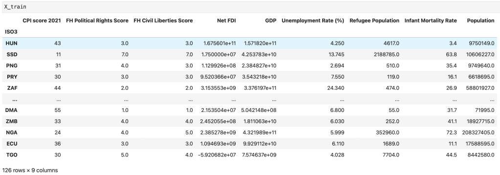
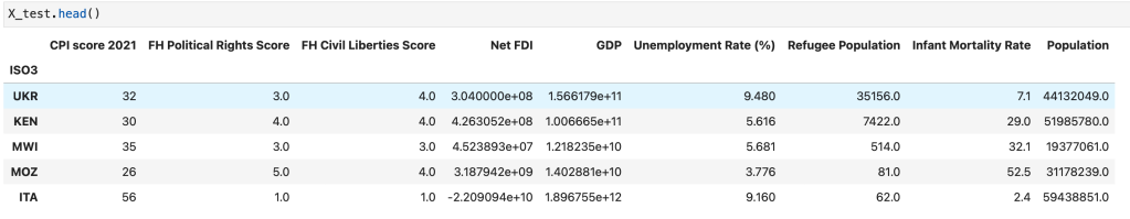
The training set is the portion of the data used to train or build the model, while the testing set is the set that evaluates the model’s performance. The ‘train_test_split’ function within the Sci-Kit Learn library partitioned the data into training and testing sets. The test set contained 25% of the data (42 countries), and the remaining 75% constituted the training set (126 countries). The testing set is usually a subset of the data the model has not seen during training. The training and testing sets are necessarily disjoint to prevent the model from memorizing the training data instead of learning the underlying patterns. If the testing set overlaps with the training set, the model may perform well on the test set but fail to generalize to new, unseen data. This failure to generalize to new data is called overfitting. Therefore, splitting the data into training and testing sets is vital to ensuring that the model is trained on one set and tested on another. The train-test split allows the model to learn from the training set while providing an unbiased evaluation of its performance on the testing set.

Code

Download Python File

Results

This section of the project required the construction of three tree-based models, a simple decision tree without any hyperparameter tuning, a decision tree with hyperparameter tuning, and a random forest.

The initial, untuned decision tree used sklearn’s default hyperparameters for the DecisionTreeClassifier method:

Gini criterion
No maximum tree depth
No maximum number of features to consider when looking for the best split

This tree resulted in an accuracy of 0.667 and the following confusion matrix.

Next, grid search with cross-validation resulted in the following optimal hyperparameters for the second decision tree:

Entropy criterion
At most seven levels in the tree
Only consider $log_2(d)$ features when looking for best split

The tuned decision tree produced an accuracy of 0.738, higher than the accuracy of the simple decision tree.

Finally, tuning for the random forest produced the following hyperparameters:

Entropy criterion
50 trees
Only consider $\sqrt{d}$ features when looking for best split

The decision tree performed the best out of the three tree models with an accuracy of 0.810.

Conclusions

From the results above, we can see that, out of the three tree-based methods, the random forest classifier performed the best on the testing data. Additionally, using entropy as the splitting criterion generally resulted in more accurate models. In the context of this project, decision trees prove to be very useful due to their ease of interpretation. Researchers can use decision trees, like the ones constructed in this project, to uncover significant variables that stimulate aid from donor governments. The decision tree produced some expected results, such as the association between high refugee populations and more foreign aid donations. Interestingly, the decision tree results imply the United States is more willing to send development aid to countries with more corruption and fewer political rights. The results from this project serve as an example of the benefit decision trees can provide to this line of research.