Support Vector Machines

Overview

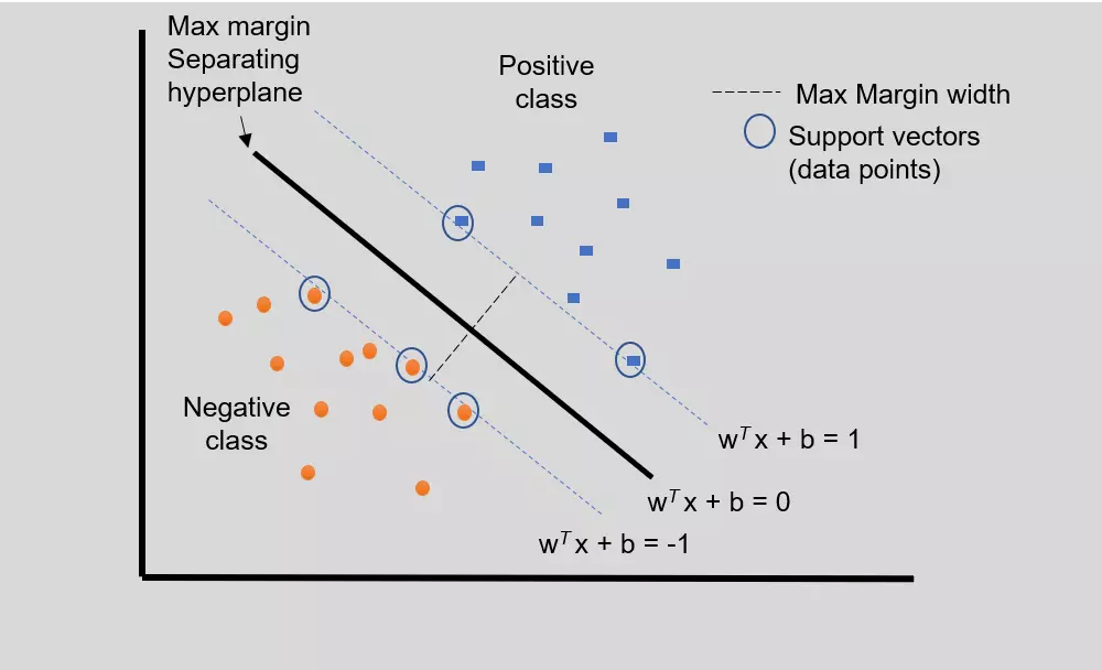
Support Vector Machines (SVMs) are a popular algorithm for classification and regression tasks. SVMs use the concept of support vectors, which are the data points closest to the decision boundary. SVMs are linear separators that aim to find the hyperplane that best separates the different classes in a high-dimensional space. In this context, the “best” decision boundary is the hyperplane that maximizes the margin between support vectors. The SVM uses the separating hyperplane to classify the data into one of two classes depending on which side of the decision boundary the data vectors lie. A single SVM can only perform binary classification tasks. Therefore, multiclass classification requires two or more SVMs depending on the number of classes.

Kernels

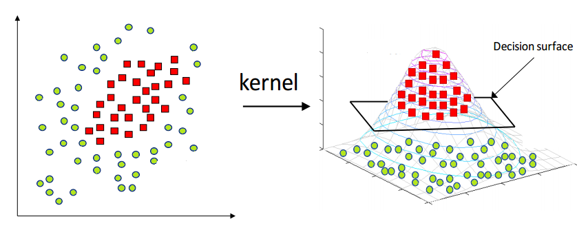
The kernel is an essential concept in SVMs, allowing them to perform nonlinear classification. The kernel function takes in a pair of data points and calculates a similarity measure between them. This similarity measure projects the data into a higher-dimensional space where it becomes linearly separable. The dot product is critical to kernel functions because it measures the similarity between two points in the original vector space. The dot product is useful because it can be computed efficiently in a higher-dimensional space.

The two most common kernel functions used in SVMs are the polynomial kernel and the radial basis function (RBF) kernel. For $d$ -degree polynomials, the polynomial kernel is defined:

$K(\mathbf{x_1}, \mathbf{x_2}) = (\mathbf{x_1}^T\mathbf{x_2} + r)^d$

where $\mathbf{x_1}$ and $\mathbf{x_2}$ are input data points and $r$ is the coefficient of the polynomial, a constant. The RBF kernel is defined:

$K(\mathbf{x_1}, \mathbf{x_2}) = \exp\left\{-\gamma||\mathbf{x_1}-\mathbf{x_2}||^2\right\}$

Polynomial Kernel Example

Consider the following 2-D data:

ID	Height (cm)	Weight (lbs)
a	175.3	199.7
b	161.3	170.9

For a polynomial kernel with degree 2 and r = 1:

$K(\mathbf{a}, \mathbf{b}) = (\mathbf{a}^T\mathbf{b} + 1)^2$

$= \left(\left[a_1b_1 + a_2b_2\right] + 1 \right)^2$

$= \left[a_1b_1 + a_2b_2\right]^2 + 2[a_1b_1 + a_2b_2] + 1$

$= [a_1b_1]^2 + 2[a_1b_1a_2b_2] + [a_2b_2]^2+ 2[a_1b_1] + 2[a_2b_2] + 1$

$= \begin{pmatrix}a_1^2\\a_1a_2\\a_2a_1 \\a_2^2\\a_1\\a_1\\a_2\\a_2\\ 1\end{pmatrix} \cdot \begin{pmatrix}b_1^2\\b_1b_2\\b_2b_1 \\b_2^2\\b_1\\b_1\\b_2\\b_2\\ 1\end{pmatrix}$

$= \begin{pmatrix}175.3^2\\(175.3)(199.7)\\(199.7)(175.3) \\199.7^2\\175.3\\175.3\\199.7\\199.7\\ 1\end{pmatrix} \cdot \begin{pmatrix}161.3^2\\(161.3)(170.9)\\(170.9)(161.3) \\170.9^2\\161.3\\161.3\\170.9\\170.9\\ 1\end{pmatrix}$

Here we can see that $\mathbf{a}$ and $\mathbf{b}$ are cast into $\mathbb{R}^9$ (9-dimensional) space.

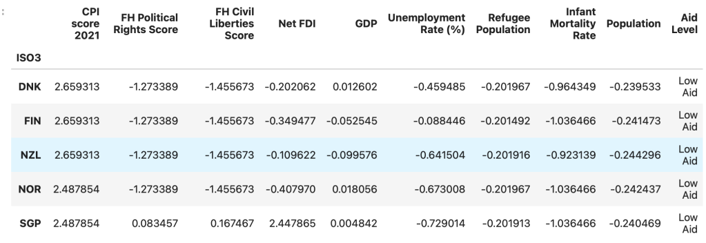
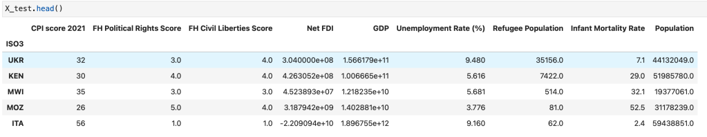
Data Prep

Supervised machine learning algorithms, such as support vector machines, require labeled data because they learn from already classified or labeled examples. The goal is to discover the mapping between the input data and the corresponding output labels. In supervised learning, the algorithm tries to find patterns in the labeled data to make predictions or classifications on new, unlabeled data.

SVM Dataset

Training and Testing Sets

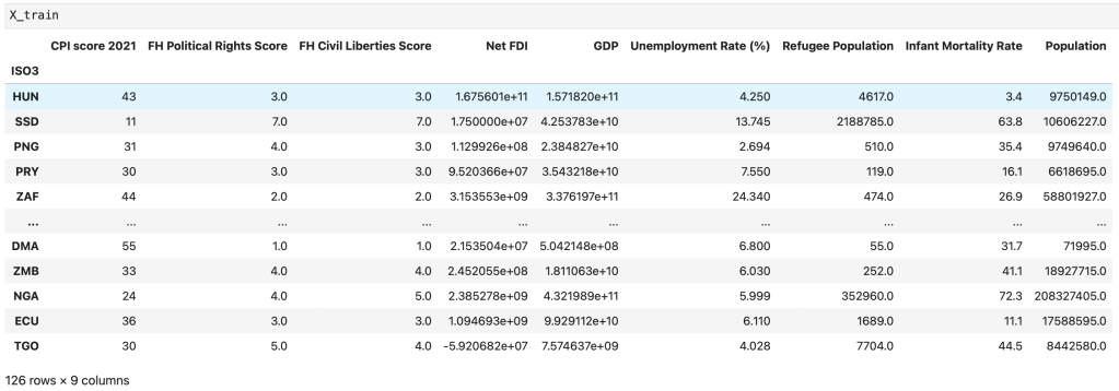
The training set is the portion of the data used to train or build the model, while the testing set is the set that evaluates the model’s performance. The testing set is usually a subset of the data the model has not seen during training. The ‘train_test_split’ function within the Sci-Kit Learn library partitioned the data into training and testing sets. The test set contained 25% of the data (42 countries), and the remaining 75% constituted the training set (127 countries). The training and testing sets are necessarily disjoint to prevent the model from memorizing the training data instead of learning the underlying patterns. If the testing set overlaps with the training set, the model may perform well on the test set but fail to generalize to new, unseen data. This failure to generalize to new data is called overfitting. Therefore, splitting the data into training and testing sets is vital to ensuring that the model is trained on one set and tested on another. The train-test split allows the model to learn from the training set while providing an unbiased evaluation of its performance on the testing set.

Code

Python Code

Results

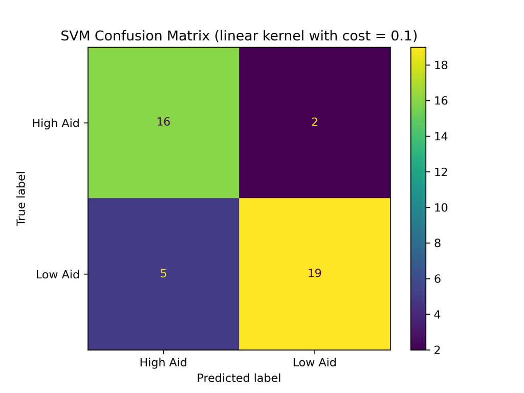
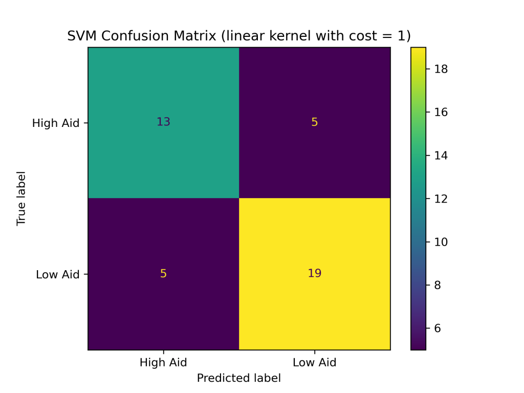
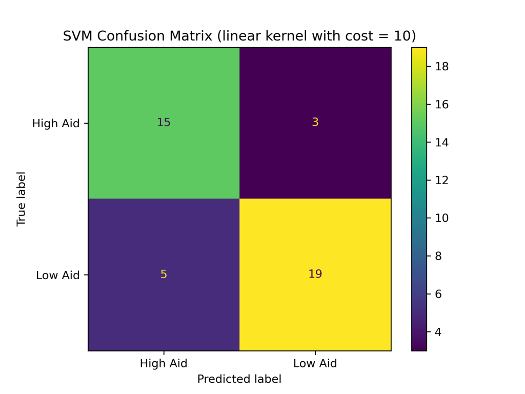
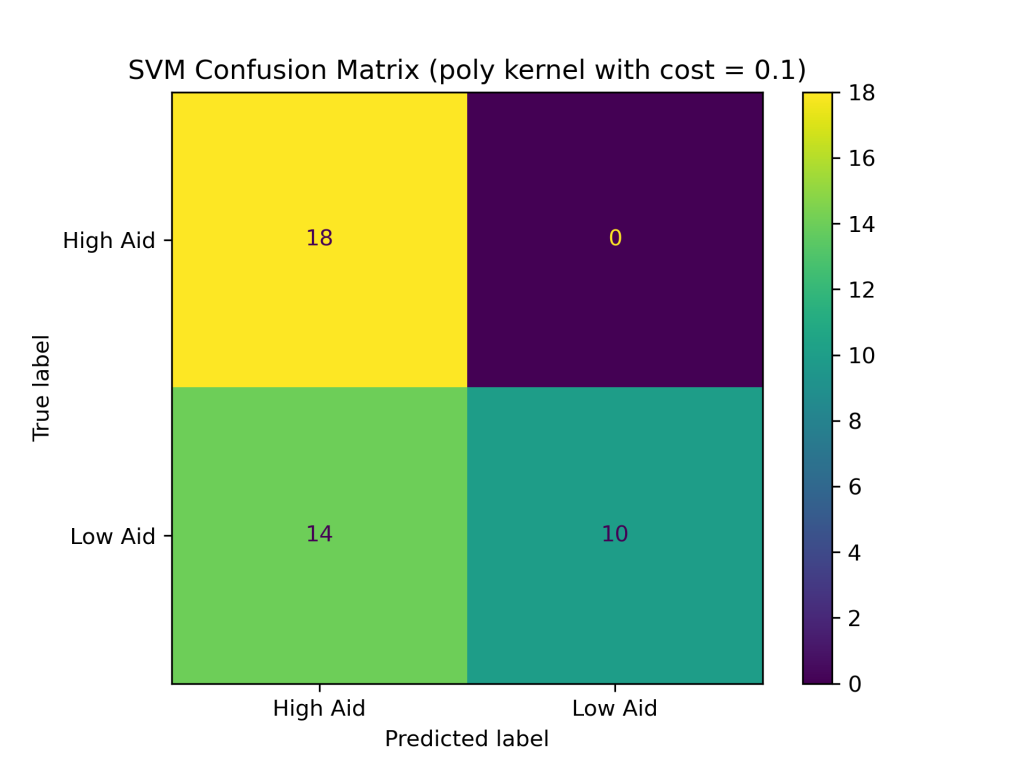
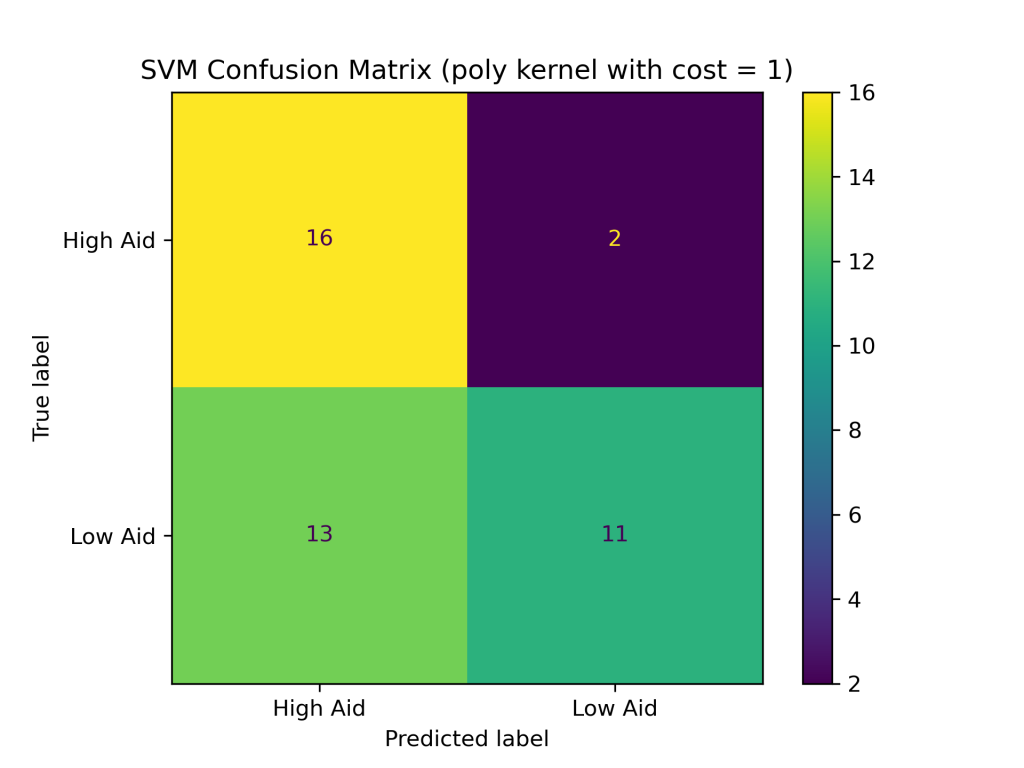
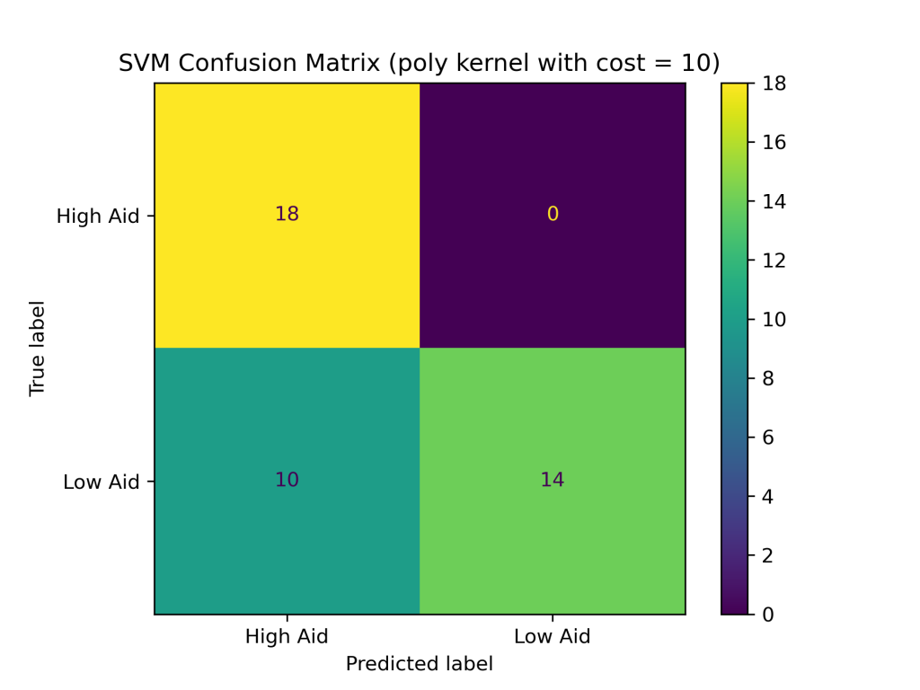
The SVM classifier with combinations of linear, polynomial, and RBF kernels with costs of 0.1, 1, and 10 produced the following test accuracies and confusion matrices:

Linear Kernel
- with cost of 0.1: 83.33%
- with cost of 1: 76.19%
- with cost of 10: 80.95%
Polynomial Kernel
- with cost of 0.1: 66.67%
- with cost of 1: 64.29%
- with cost of 10: 76.19%
RBF Kernel
- with cost of 0.1: 83.33%
- with cost of 1: 88.10%
- with cost of 10: 83.33%

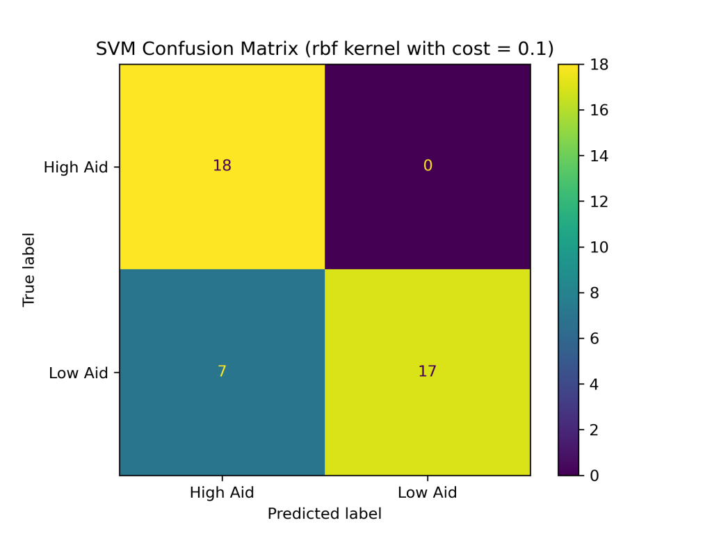
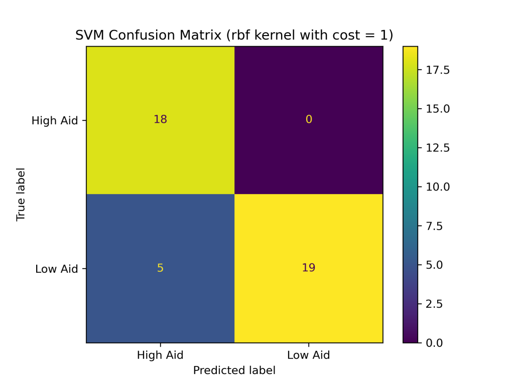
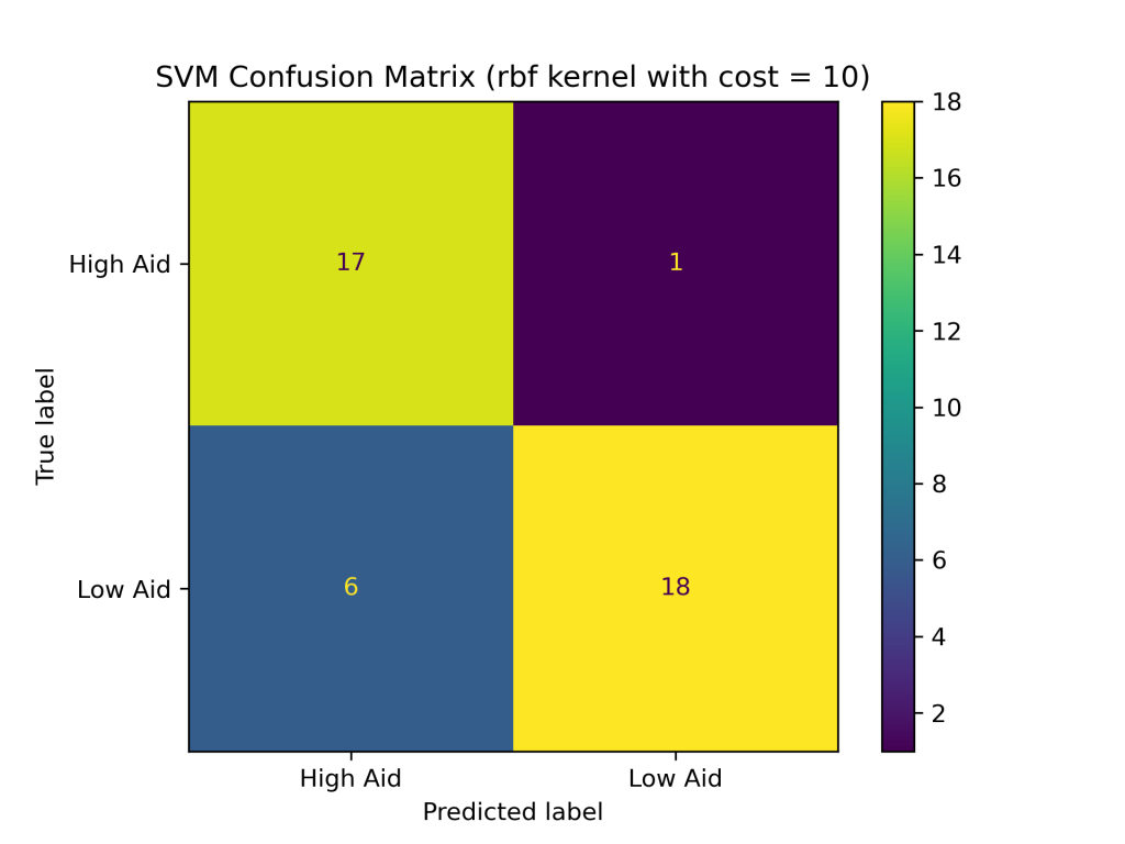
Conclusions

The above results show that the RBF kernel generally performed better on the foreign aid data than the linear and polynomial kernels. The higher accuracy of the SVM with the RBF kernel suggests that it is better at handling complex and non-linear relationships between the input variables and output classes in the foreign aid data. Additionally, the SVM with an RBF kernel and a cost of 1 produced the highest accuracy of the nine SVM classifiers constructed, with a testing accuracy of about 88%.In addition to having the highest test accuracy among SVM models, the SVM with an RBF kernel and cost = 1 performed better than the naive Bayes and decision tree classifiers evaluated earlier in this project. Thus far, SVMs are the best supervised learning model in predicting U.S. foreign aid allocation patterns.